DuckDB in R

1 Establish a connection to DuckDB

Code

library(tidyverse)
library(gt)
library(DBI)
library(duckdb)
library(duckplyr)
library(tictoc)
library(nycflights23)

Code

# to start an in-memory database
con <- dbConnect(duckdb())
# or con <- dbConnect(duckdb(), dbdir = ":memory:")

# to use a database file (not shared between processes)
# con <- dbConnect(duckdb(), dbdir = "my-db.duckdb", read_only = FALSE)
# to use a database file (shared between processes)
# con <- dbConnect(duckdb(), dbdir = "my-db.duckdb", read_only = TRUE)

2 Load data into DuckDB

2.1 Load data from `R` chunk

Code

# write mtcars, from R environment, to duckdb database
dbWriteTable(con, "mtcars", mtcars) 

# register iris, from R environment, as a view in duckdb
duckdb_register(con, "view", iris) 
duckdb_register(con, "flights", flights)

# read data from local file to duckdb
duckdb_read_csv(con, "gdp", "data/gdp.csv", na.strings = "NA")

2.2 Load data from `sql` chunk

Code

create table gdp2 as
select * from read_csv('data/gdp.csv')

2.3 Show tables in DuckDB

list tables in R chunk

Code

dbListTables(con)

[1] "flights" "gdp"     "gdp2"    "mtcars"  "view"

list tables in sql connection chunk

Code

show tables

5 records
name
flights
gdp
gdp2
mtcars
view

3 Query data from DuckDB

3.1 Oder of query execution

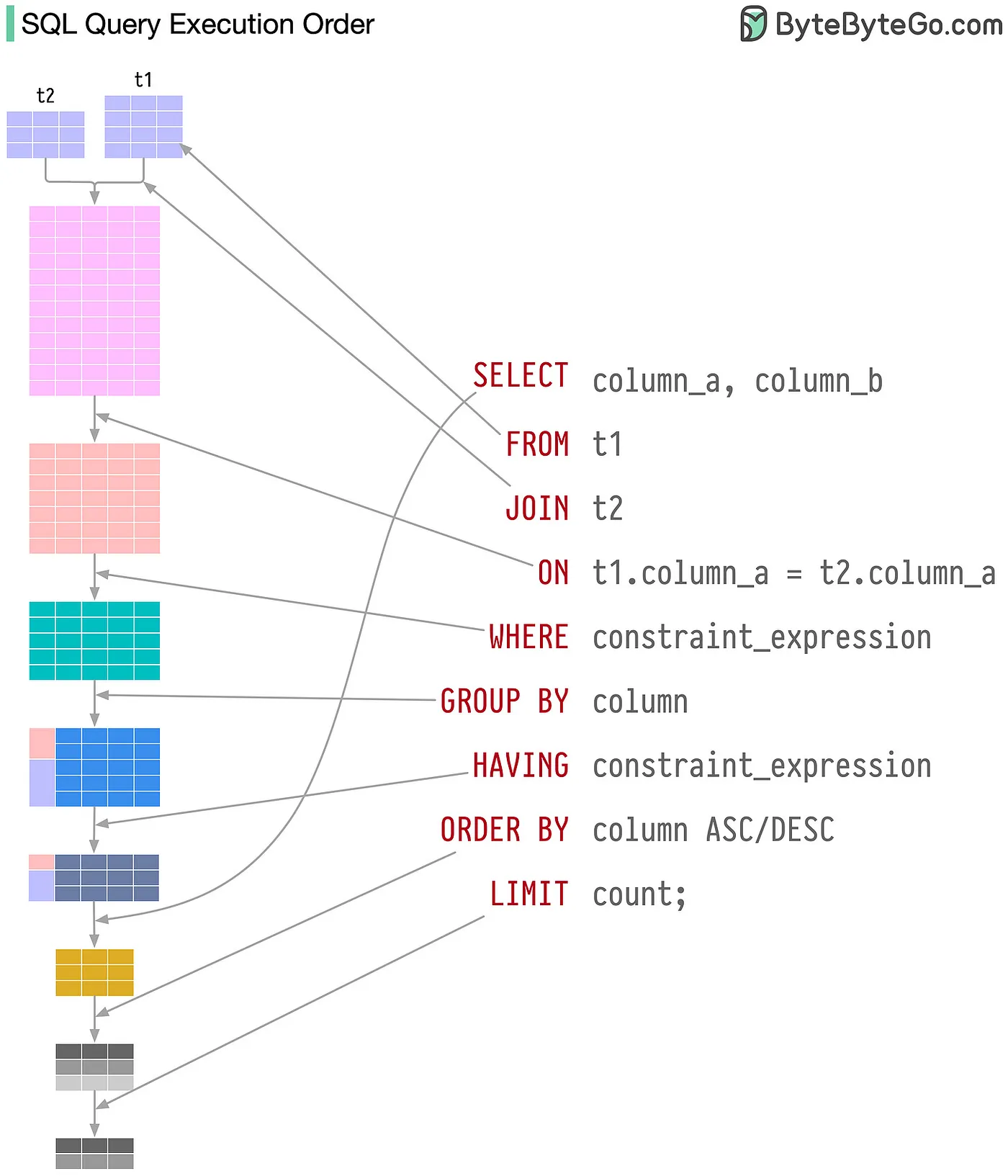
Please visit SQL Query Order for more information.

3.2 View the whole table

Code

SELECT * FROM gdp

Displaying records 1 - 10
X	country_name	scode	COWcode	year	gdppc	edu_year
1	Mexico	MEX	70	1946	3.174	2.292
2	Mexico	MEX	70	1947	3.242	2.354
3	Mexico	MEX	70	1948	3.366	2.416
4	Mexico	MEX	70	1949	3.568	2.478
5	Mexico	MEX	70	1950	3.960	2.540
6	Mexico	MEX	70	1951	4.181	2.628
7	Mexico	MEX	70	1952	4.288	2.716
8	Mexico	MEX	70	1953	4.306	2.804
9	Mexico	MEX	70	1954	4.469	2.892
10	Mexico	MEX	70	1955	4.644	2.980

3.3 More complex queries

Code

select * from mtcars
where hp > 100
order by -hp

Displaying records 1 - 10
mpg	cyl	disp	hp	drat	wt	qsec	am	gear	carb
15.0	8	301.0	335	3.54	3.570	14.60	1	5	8
15.8	8	351.0	264	4.22	3.170	14.50	1	5	4
14.3	8	360.0	245	3.21	3.570	15.84	0	3	4
13.3	8	350.0	245	3.73	3.840	15.41	0	3	4
14.7	8	440.0	230	3.23	5.345	17.42	0	3	4
10.4	8	460.0	215	3.00	5.424	17.82	0	3	4
10.4	8	472.0	205	2.93	5.250	17.98	0	3	4
16.4	8	275.8	180	3.07	4.070	17.40	0	3	3
17.3	8	275.8	180	3.07	3.730	17.60	0	3	3
15.2	8	275.8	180	3.07	3.780	18.00	0	3	3

We can omit Select * in the query in duckdb as it is the default.

Code

from mtcars
where hp > 100
order by -hp

Displaying records 1 - 10
mpg	cyl	disp	hp	drat	wt	qsec	am	gear	carb
15.0	8	301.0	335	3.54	3.570	14.60	1	5	8
15.8	8	351.0	264	4.22	3.170	14.50	1	5	4
14.3	8	360.0	245	3.21	3.570	15.84	0	3	4
13.3	8	350.0	245	3.73	3.840	15.41	0	3	4
14.7	8	440.0	230	3.23	5.345	17.42	0	3	4
10.4	8	460.0	215	3.00	5.424	17.82	0	3	4
10.4	8	472.0	205	2.93	5.250	17.98	0	3	4
16.4	8	275.8	180	3.07	4.070	17.40	0	3	3
17.3	8	275.8	180	3.07	3.730	17.60	0	3	3
15.2	8	275.8	180	3.07	3.780	18.00	0	3	3

We can anti-select columns in the query in duckdb as shown below.

Code

from flights
select * exclude (year, month, day)
where month = 1 and day = 1
order by dep_delay desc
limit 10

Displaying records 1 - 10
dep_time	sched_dep_time	dep_delay	arr_time	sched_arr_time	arr_delay	carrier	flight	tailnum	origin	dest	air_time	distance	hour	minute	time_hour
1733	1045	408	2018	1345	393	UA	740	N17730	EWR	MCO	127	937	10	45	2023-01-01 10:00:00
1445	830	375	1754	1205	349	DL	126	N705TW	JFK	SAN	330	2446	8	30	2023-01-01 08:00:00
1453	840	373	1735	1156	339	B6	968	N193JB	LGA	PBI	147	1035	8	40	2023-01-01 08:00:00
1158	600	358	1404	831	333	DL	825	N3756	EWR	ATL	108	746	6	0	2023-01-01 06:00:00
1124	600	324	1320	755	325	DL	487	N394DX	LGA	DTW	87	502	6	0	2023-01-01 06:00:00
1933	1420	313	2214	1731	283	B6	656	N2086J	EWR	MCO	130	937	14	20	2023-01-01 14:00:00
2030	1545	285	2304	1856	248	UA	789	N77259	LGA	IAH	185	1416	15	45	2023-01-01 15:00:00
1115	639	276	1402	940	262	B6	112	N2086J	EWR	MCO	140	937	6	39	2023-01-01 06:00:00
1056	700	236	1345	1027	198	AS	349	N268AK	EWR	SEA	331	2402	7	0	2023-01-01 07:00:00
2127	1735	232	2247	1900	227	B6	494	N2102J	JFK	ROC	55	264	17	35	2023-01-01 17:00:00

More complex queries can be written in sql chunk as shown below.

Code

SELECT *
FROM (
   SELECT
     tailnum,
    COUNT(*) AS count,
    AVG(distance) AS dist,
    AVG(arr_delay) AS delay
  FROM flights
  GROUP BY tailnum
) q01
WHERE (count > 20.0) AND (dist < 2000.0) AND (NOT((delay IS NULL)))
limit 10

Displaying records 1 - 10
tailnum	count	dist	delay
N925AN	70	987.4000	-1.771429
N2043J	164	1702.0427	20.331210
N659JB	222	1174.3964	16.052885
N342NW	73	1015.0548	7.478873
N612NK	64	1130.4375	3.645161
N2027J	122	1432.7787	26.547826
N24715	173	915.2717	7.093567
N413UA	80	914.5375	12.126582
N27274	234	1323.9359	5.914163
N73256	99	1072.1414	7.232323

4 Save outcome of query into R environment

We can save the outcome of the query into the R environment as shown below¹.

Code

tic("sql")

Code

SELECT tailnum, AVG(distance) AS dist, AVG(arr_delay) AS delay
FROM flights
WHERE month = 1
GROUP BY tailnum
HAVING COUNT(*) > 20
ORDER BY delay DESC
LIMIT 10

Code

toc()

sql: 0.034 sec elapsed

Code

tic("R")

Code

toc()

R: 0.091 sec elapsed

The outcome of the query is saved in the R environment as top10_delayed_planes and we can call it in R chunk as shown below.

Code

# same result with the query in R
top10_delayed_planes |> 
  gt() |> 
  tab_options(table.width = pct(90),
              column_labels.font.size = 16,
              column_labels.font.weight = "bold",
              column_labels.text_transform = "capitalize") |>
  opt_row_striping()

tailnum	dist	delay
N394DA	1224.1333	47.43333
N325PQ	423.8214	44.89286
N691CA	417.5641	44.02857
N272PQ	502.4242	33.12121
N320SY	544.0833	32.08333
N558JB	1127.8400	32.00000
N116AN	2506.3333	31.44444
N187GJ	545.8182	30.87879
N905XJ	458.5714	30.57143
N193JB	448.6078	29.98000

Why bother with duckdb when we can do the same in R? You might ask. The answer is that duckdb is faster than R for large datasets. As showed above, the query in duckdb is much faster than in R to get the same results.

We might not notice a significant difference in query execution speed in this example because the dataset is small. However, the discrepancy becomes more apparent with larger datasets. Let’s examine a big dataset to observe the contrast in query execution speed. We’ll use a dataset containing item checkouts from Seattle public libraries, accessible online at Seattle.

When attempting to read the dataset with read_csv(), it may encounter considerable processing delays or even fail outright. This is primarily due to the dataset’s substantial size, comprising approximately 41,389,465 rows, spanning 12 columns, and occupying 9.21 GB of storage space. The following code would fail to read such voluminous data.

```{r}
read_csv("~/GitHub/data/seattle-library-checkouts.csv") |> 
  nrow()
```

Let’s try to query with duckdb.

Code

tic("sql")

Code

Select Count(*)
From read_csv('~/GitHub/data/seattle-library-checkouts.csv')

1 records
count_star()
41389465

Code

toc()

sql: 8.173 sec elapsed

DuckDB took a bit longer to retrieve the results, more than 4 seconds, but the performance was quite acceptable. It outperformed R, which failed to read the data altogether.

5 Disconnect from DuckDB

Code

dbDisconnect(con, shutdown = TRUE)

Footnotes

Please go to upper right corner to view the source code.↩︎

1 Establish a connection to DuckDB

2 Load data into DuckDB

2.1 Load data from R chunk

2.2 Load data from sql chunk

2.3 Show tables in DuckDB

3 Query data from DuckDB

3.1 Oder of query execution

3.2 View the whole table

3.3 More complex queries

4 Save outcome of query into R environment

5 Disconnect from DuckDB

Footnotes

2.1 Load data from `R` chunk

2.2 Load data from `sql` chunk